Brian hears

Brian hears is an auditory modelling library for Python. It is part of the neural network simulator package Brian, but can also be used on its own. To download Brian hears, simply download Brian: Brian hears is included as part of the package.
Brian hears is primarily designed for generating and manipulating sounds, and applying large banks of filters. We import the package by writing:
from brian import *
from brian.hears import *
Then, for example, to generate a tone or a whitenoise we would write:
sound1 = tone(1*kHz, .1*second)
sound2 = whitenoise(.1*second)
These sounds can then be manipulated in various ways, for example:
sound = sound1+sound2
sound = sound.ramp()
If you have the pygame package installed, you can also play these sounds:
sound.play()
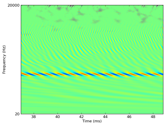
We can filter these sounds through a bank of 3000 gammatone filters covering the human auditory range as follows:
cf = erbspace(20*Hz, 20*kHz, 3000)
fb = Gammatone(sound, cf)
output = fb.process()
The output of this would look something like this (zoomed into one region):
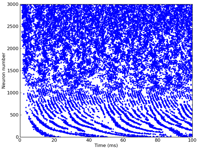
Alternatively, if we’re interested in modelling auditory nerve fibres, we could feed the output of this filterbank directly into a group of neurons defined with Brian:
# Half-wave rectification and compression [x]^(1/3)
ihc = FunctionFilterbank(fb, lambda x: 3*clip(x, 0, Inf)**(1.0/3.0))
# Leaky integrate-and-fire model with noise and refractoriness
eqs = '''
dv/dt = (I-v)/(1*ms)+0.2*xi*(2/(1*ms))**.5 : 1
I : 1
'''
anf = FilterbankGroup(ihc, 'I', eqs, reset=0, threshold=1, refractory=5*ms)
This model would give output something like this:
The human cochlea applies the equivalent of 3000 auditory filters, which causes a technical problem for modellers which this package is designed to address. At a typical sample rate, the output of 3000 filters would saturate the computer’s RAM in a few seconds. To deal with this, we use online computation, that is we only ever keep in memory the output of the filters for a relatively short duration (say, the most recent 20ms), do our modelling with these values, and then discard them. Although this requires that some models be rewritten for online rather than offline computation, it allows us to easily handle models with very large numbers of channels. 3000 or 6000 for human monaural or binaural processing is straightforward, and even much larger banks of filters can be used (for example, around 30,000 in Goodman DFM, Brette R (2010). Spike-timing-based computation in sound localization. PLoS Comput. Biol. 6(11): e1000993. doi:10.1371/journal.pcbi.1000993). Techniques for online computation are discussed below in the section Online computation.
Brian hears consists of classes and functions for defining sounds, filter chains, cochlear models, neuron models and head-related transfer functions. These classes are designed to be modular and easily extendable. Typically, a model will consist of a chain starting with a sound which is plugged into a chain of filter banks, which are then plugged into a neuron model.
The two main classes in Brian hears are Sound and Filterbank,
which function very similarly. Each consists of multiple channels (typically
just 1 or 2 in the case of sounds, and many in the case of filterbanks,
but in principle any number of channels is possible for either). The difference
is that a filterbank has an input source, which can be either a sound or
another filterbank.
All scripts using Brian hears should start by importing the Brian and Brian hears packages as follows:
from brian import *
from brian.hears import *
To download Brian hears, simply download Brian: Brian hears is included as part of the package.
See also
Reference documentation for Brian hears, which covers everything in this overview in detail, and more. List of examples of using Brian hears.
Sounds
Sounds can be loaded from a WAV or AIFF file with the loadsound()
function (and saved with the savesound() function or Sound.save()
method), or by initialising with a filename:
sound = loadsound('test.wav')
sound = Sound('test.aif')
sound.save('test.wav')
Various standard types of sounds can also be constructed, e.g. pure tones, white noise, clicks and silence:
sound = tone(1*kHz, 1*second)
sound = whitenoise(1*second)
sound = click(1*ms)
sound = silence(1*second)
You can pass a function of time or an array to initialise a sound:
# Equivalent to Sound.tone
sound = Sound(lambda t:sin(50*Hz*2*pi*t), duration=1*second)

# Equivalent to Sound.whitenoise
sound = Sound(randn(int(1*second*44.1*kHz)), samplerate=44.1*kHz)
Multiple channel sounds can be passed as a list or tuple of filenames,
arrays or Sound objects:
sound = Sound(('left.wav', 'right.wav'))
sound = Sound((randn(44100), randn(44100)), samplerate=44.1*kHz)
sound = Sound((Sound.tone(1*kHz, 1*second),
               Sound.tone(2*kHz, 1*second)))
A multi-channel sound is also a numpy array of shape (nsamples, nchannels),
and can be initialised as this (or converted to a standard numpy array):
sound = Sound(randn(44100, 2), samplerate=44.1*kHz)
arr = array(sound)
Sounds can be added and multiplied:
sound = Sound.tone(1*kHz, 1*second)+0.1*Sound.whitenoise(1*second)
For more details on combining and operating on sounds, including shifting them
in time, repeating them, resampling them, ramping them, finding and setting
intensities, plotting spectrograms, etc., see Sound.
Sounds can be played using the play() function or Sound.play() method:
play(sound)
sound.play()
Sequences of sounds can be played as:
play(sound1, sound2, sound3)
The number of channels in a sound can be found using the nchannels
attribute, and individual channels can be extracted using the
Sound.channel() method, or using the left and right attributes
in the case of stereo sounds:
print sound.nchannels
print amax(abs(sound.left-sound.channel(0)))
As an example of using this, the following swaps the channels in a stereo sound:
sound = Sound('test_stereo.wav')
swappedsound = Sound((sound.right, sound.left))
swappedsound.play()
The level of the sound can be computed and changed with the sound.level
attribute. Levels are returned in dB which is a special unit in Brian hears.
For example, 10*dB+10 will raise an error because 10 does not have
units of dB. The multiplicative gain of a value in dB can be computed with
the function gain(level). All dB values are measured as RMS dB SPL assuming
that the values of the sound object are measured in Pascals. Some examples:
sound = whitenoise(100*ms)
print sound.level
sound.level = 60*dB
sound.level += 10*dB
sound *= gain(-10*dB)
Filter chains
The standard way to set up a model based on filterbanks is to start with a sound and then construct a chain of filterbanks that modify it, for example a common model of cochlear filtering is to apply a bank of gammatone filters, and then half wave rectify and compress it (for example, with a 1/3 power law). This can be achieved in Brian hears as follows (for 3000 channels in the human hearing range from 20 Hz to 20 kHz):
cfmin, cfmax, cfN = 20*Hz, 20*kHz, 3000
cf = erbspace(cfmin, cfmax, cfN)
sound = Sound('test.wav')
gfb = GammatoneFilterbank(sound, cf)
ihc = FunctionFilterbank(gfb, lambda x: clip(x, 0, Inf)**(1.0/3.0))
The erbspace() function constructs an array of centre frequencies on the
ERB scale. The GammatoneFilterbank(source, cf) class creates a bank
of gammatone filters with inputs coming from source and the centre
frequencies in the array cf. The FunctionFilterbank(source, func)
creates a bank of filters that applies the given function func to the inputs
in source.
Filterbanks can be added and multiplied, for example for creating a linear and nonlinear path, e.g.:
sum_path_fb = 0.1*linear_path_fb+0.2*nonlinear_path_fb
A filterbank must have an input with either a single channel or an equal number
of channels. In the former case, the single channel is duplicated for each of
the output channels. However, you might want to apply gammatone filters to a
stereo sound, for example, but in this case it’s not clear how to duplicate
the channels and you have to specify it explicitly. You can do this using the
Repeat, Tile, Join and Interleave
filterbanks. For example, if the input is a stereo sound
with channels LR then you can get an output with channels LLLRRR or LRLRLR
by writing (respectively):
fb = Repeat(sound, 3)
fb = Tile(sound, 3)
To combine multiple filterbanks into one, you can either join them in series or interleave them, as follows:
fb = Join(source1, source2)
fb = Interleave(source1, source2)
For a more general (but more complicated) approach, see
RestructureFilterbank.
Two of the most important generic filterbanks (upon which many of the others
are based) are LinearFilterbank and FIRFilterbank. The former
is a generic digital filter for FIR and IIR filters. The latter is specifically
for FIR filters. These can be implemented with the former, but the
implementation is optimised using FFTs with the latter (which can often be
hundreds of times faster, particularly for long impulse responses). IIR filter
banks can be designed using IIRFilterbank which is based on the
syntax of the iirdesign scipy function.
You can change the input source to a Filterbank by modifying its
source attribute, e.g. to change the input sound of a filterbank fb
you might do:
fb.source = newsound
Note that the new source should have the same number of channels.
You can implement control paths (using the output of one filter chain path
to modify the parameters of another filter chain path) using
ControlFilterbank (see reference documentation for more details).
For examples of this in action, see the following:
Connecting with Brian
To create spiking neuron models based on filter chains, you use the
FilterbankGroup class. This acts exactly like a standard Brian
NeuronGroup except that you give a source filterbank and choose
a state variable in the target equations for the output of the filterbank.
A simple auditory nerve fibre model would take the inner hair cell model from
earlier, and feed it into a noisy leaky integrate-and-fire model as follows:
# Inner hair cell model as before
cfmin, cfmax, cfN = 20*Hz, 20*kHz, 3000
cf = erbspace(cfmin, cfmax, cfN)
sound = Sound.whitenoise(100*ms)
gfb = Gammatone(sound, cf)
ihc = FunctionFilterbank(gfb, lambda x: 3*clip(x, 0, Inf)**(1.0/3.0))
# Leaky integrate-and-fire model with noise and refractoriness
eqs = '''
dv/dt = (I-v)/(1*ms)+0.2*xi*(2/(1*ms))**.5 : 1
I : 1
'''
G = FilterbankGroup(ihc, 'I', eqs, reset=0, threshold=1, refractory=5*ms)
# Run, and raster plot of the spikes
M = SpikeMonitor(G)
run(sound.duration)
raster_plot(M)
show()
And here’s the output (after 6 seconds of computation on a 2GHz laptop):
Plotting
Often, you want to use log-scaled axes for frequency in plots, but the
built-in matplotlib axis labelling for log-scaled axes doesn’t work well for
frequencies. We provided two functions (log_frequency_xaxis_labels() and
log_frequency_yaxis_labels()) to automatically set useful axis labels.
For example:
cf = erbspace(100*Hz, 10*kHz)
...
semilogx(cf, response)
axis('tight')
log_frequency_xaxis_labels()
Online computation
Typically in auditory modelling, we precompute the entire output of each
channel of the filterbank (“offline computation”), and then work with that.
This is straightforward,
but puts a severe limit on the number of channels we can use or the length of
time we can work with (otherwise the RAM would be quickly exhausted).
Brian hears allows us to use a very large number of channels in filterbanks,
but at the cost of only storing the output of the filterbanks for a relatively
short period of time (“online computation”).
This requires a slight change in the way we use the
output of the filterbanks, but is actually not too difficult. For example,
suppose we wanted to compute the vector of RMS values for each channel of the
output of the filterbank. Traditionally, or if we just use the syntax
output = fb.process() in Brian hears, we have an array output of
shape (nsamples, nchannels). We could compute the vector of RMS values as:
rms = sqrt(mean(output**2, axis=0))
To do the same thing with online computation, we simply store a vector of the running sum of squares, and update it for each buffered segment as it is computed. At the end of the processing, we divide the sum of squares by the number of samples and take the square root.
The Filterbank.process()
method allows us to pass an optional function f(output, running) of
two arguments. In this case, process() will first call
running = f(output, 0) for the first buffered segment output. It will
then call running = f(output, running) for each subsequent segment. In
other words, it will “accumulate” the output of f, passing the output of
each call to the subsequent call. To compute the vector of RMS values then,
we simply do:
def sum_of_squares(input, running):
    return running+sum(input**2, axis=0)

rms = sqrt(fb.process(sum_of_squares)/nsamples)
If the computation you wish to perform is more complicated than can be
achieved with the process() method, you can derive a class
from Filterbank (see that class’ reference documentation for more
details on this).
Buffering interface
The Sound, OnlineSound and Filterbank classes
(and all classes derived from them) all implement the same buffering
mechanism. The purpose of this is to allow for efficient processing of
multiple channels in buffers. Rather than precomputing the application of
filters to all channels (which for large numbers of channels or long sounds
would not fit in memory), we process small chunks at a time. The entire design
of these classes is based on the idea of buffering, as defined by the base
class Bufferable (see section Options).
Each class
has two methods, buffer_init() to initialise the buffer, and
buffer_fetch(start, end) to fetch the portion of the buffer from samples
with indices from start to end (not including end as standard for
Python). The buffer_fetch(start, end) method should return a 2D array of
shape (end-start, nchannels) with the buffered values.
From the user point of view, all you need to do, having set up a chain of
Sound and Filterbank objects, is to call buffer_fetch(start, end)
repeatedly. If the output of a Filterbank is being plugged into a
FilterbankGroup object, everything is handled automatically. For cases
where the number of channels is small or the length of the input source is short,
you can use the Filterbank.fetch(duration)() method to automatically
handle the initialisation and repeated application of buffer_fetch.
To extend Filterbank, it is often sufficient just to implement the
buffer_apply(input) method. See the documentation for Filterbank
for more details.
Library
Brian hears comes with a package of predefined filter classes to be used as basic blocks by the user. All of them are implemented as filterbanks.
First, a series of standard filters widely used in audio processing are available:
| Class | Descripition | Example |
|---|---|---|
IIRFilterbank |
Bank of low, high, bandpass or bandstop filter of type Chebyshef, Elliptic, etc... | Example: IIRfilterbank (hears) |
Butterworth |
Bank of low, high, bandpass or bandstop Butterworth filters | Example: butterworth (hears) |
LowPass |
Bank of lowpass filters of order 1 | Example: cochleagram (hears) |
Second, the library provides linear auditory filters developed to model the middle ear transfer function and the frequency analysis of the cochlea:
| Class | Description | Example |
|---|---|---|
MiddleEar |
Linear bandpass filter, based on middle-ear frequency response properties | Example: tan_carney_simple_test (hears/tan_carney_2003) |
Gammatone |
Bank of IIR gammatone filters (based on Slaney implementation) | Example: gammatone (hears) |
ApproximateGammatone |
Bank of IIR gammatone filters (based on Hohmann implementation) | Example: approximate_gammatone (hears) |
LogGammachirp |
Bank of IIR gammachirp filters with logarithmic sweep (based on Irino implementation) | Example: log_gammachirp (hears) |
LinearGammachirp |
Bank of FIR chirp filters with linear sweep and gamma envelope | Example: linear_gammachirp (hears) |
LinearGaborchirp |
Bank of FIR chirp filters with linear sweep and gaussian envelope |
Finally, Brian hears comes with a series of complex nonlinear cochlear models developed to model nonlinear effects such as filter bandwith level dependency, two-tones suppression, peak position level dependency, etc.
| Class | Description | Example |
|---|---|---|
DRNL |
Dual resonance nonlinear filter as described in Lopez-Paveda and Meddis, JASA 2001 | Example: drnl (hears) |
DCGC |
Compressive gammachirp auditory filter as described in Irino and Patterson, JASA 2001 | Example: dcgc (hears) |
TanCarney |
Auditory phenomenological model as described in Tan and Carney, JASA 2003 | Example: tan_carney_simple_test (hears/tan_carney_2003) |
ZhangSynapse |
Model of an inner hair cell – auditory nerve synapse (Zhang et al., JASA 2001) | Example: tan_carney_simple_test (hears/tan_carney_2003) |
Head-related transfer functions
You can work with head-related transfer functions (HRTFs) using the three
classes HRTF (a single pair of left/right ear HRTFs),
HRTFSet (a set of HRTFs, typically for a single individual), and
HRTFDatabase (for working with databases of individuals). At the
moment, we have included only one HRTF database, the IRCAM_LISTEN
public HRTF database. However, we will add support for the CIPIC and MIT-KEMAR
databases in a subsequent release. There is also one artificial HRTF database,
HeadlessDatabase used for generating HRTFs of artifically introduced ITDs.
An example of loading the IRCAM database, selecting a subject and plotting the pair of impulse responses for a particular direction:
hrtfdb = IRCAM_LISTEN(r'F:\HRTF\IRCAM')
hrtfset = hrtfdb.load_subject(1002)
hrtf = hrtfset(azim=30, elev=15)
plot(hrtf.left)
plot(hrtf.right)
show()
HRTFSet has a set of coordinates, which can be
accessed via the coordinates attribute, e.g.:
print hrtfset.coordinates['azim']
print hrtfset.coordinates['elev']
You can also generated filterbanks associated either to an HRTF or
an entire HRTFSet. Here is an example of doing this with the IRCAM
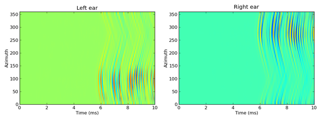
database, and applying this filterbank to some white noise and plotting the
response as an image:
# Load database
hrtfdb = IRCAM_LISTEN(r'D:\HRTF\IRCAM')
hrtfset = hrtfdb.load_subject(1002)
# Select only the horizontal plane
hrtfset = hrtfset.subset(lambda elev: elev==0)
# Set up a filterbank
sound = whitenoise(10*ms)
fb = hrtfset.filterbank(sound)
# Extract the filtered response and plot
img = fb.process().T
img_left = img[:img.shape[0]/2, :]
img_right = img[img.shape[0]/2:, :]
subplot(121)
imshow(img_left, origin='lower left', aspect='auto',
       extent=(0, sound.duration/ms, 0, 360))
xlabel('Time (ms)')
ylabel('Azimuth')
title('Left ear')
subplot(122)
imshow(img_right, origin='lower left', aspect='auto',
       extent=(0, sound.duration/ms, 0, 360))
xlabel('Time (ms)')
ylabel('Azimuth')
title('Right ear')
show()
This generates the following output:
For more details, see the reference documentation for HRTF,
HRTFSet, HRTFDatabase, IRCAM_LISTEN and
HeadlessDatabase.